Beyond Deployment: Mastering Embedding Drift Detection for Production LLMs

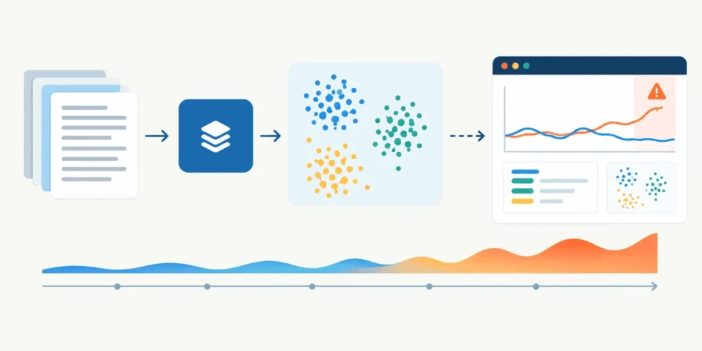
When a Large Language Model (LLM) is deployed into a production environment, the common misconception is that the development phase has concluded. In reality, the "go-live" moment is merely the beginning of a continuous lifecycle. In the real world, user behavior is fluid; it evolves, shifts, and adapts to new trends, technologies, and social contexts. As the input data changes, so too must the model’s internal numerical representation of that data—the embeddings.

For data scientists and machine learning engineers, failing to account for this evolution leads to "embedding drift." This phenomenon occurs when the statistical properties of the data entering the model change significantly from the data used during the initial training or baseline phase. If left unmonitored, drift can lead to degraded model performance, hallucinated outputs, or irrelevant retrieval results. This article explores the mechanics of embedding drift and provides a practical, code-driven roadmap to detecting it in production pipelines.

Understanding Embedding Drift: Why It Matters

Embeddings are high-dimensional vector representations of text. They translate semantic meaning into a geometric space where similar concepts are clustered together. However, these vectors are not static entities; they are highly sensitive to the distribution of the source data.

The Mechanism of Drift

Embedding drift occurs when the semantic "center of gravity" of incoming user queries moves away from the baseline established during development. Consider an e-commerce chatbot trained on customer service inquiries regarding basic account settings. If a sudden marketing campaign introduces a surge of questions about a new, experimental crypto-payment feature, the incoming embeddings will shift into a region of the vector space that the model has never been optimized to navigate.

Why Traditional Metrics Fall Short

Traditional drift detection, such as the Kolmogorov-Smirnov test or Population Stability Index (PSI), was designed for tabular data where features have clear, independent distributions. Embeddings, by contrast, are high-dimensional (often 384, 768, or 1536 dimensions). In such high-dimensional spaces, traditional statistical tests often succumb to the "curse of dimensionality," failing to capture subtle but critical changes in the underlying semantic structure. Consequently, specialized, model-based, or geometric approaches are required to maintain system integrity.

Core Techniques for Effective Drift Detection

To accurately identify when a model requires retraining or fine-tuning, practitioners typically employ one of three primary strategies:

1. Domain Classifier (Adversarial Detection): This approach treats drift detection as a binary classification problem. By training a secondary "shadow" model (such as a Random Forest) to distinguish between baseline data and live production data, we can measure the model’s performance. If the shadow model can easily tell the difference (high ROC-AUC), it implies the production data has drifted significantly.
2. Centroid Distance (Center of Mass): This geometric method calculates the mean vector (centroid) of both the baseline and production datasets. By measuring the distance between these two points, we can quantify the "shift." While computationally efficient, it is less granular than the classification approach.
3. Maximum Mean Discrepancy (MMD): A more advanced kernel-based method that compares the distributions of two datasets in a Reproducing Kernel Hilbert Space (RKHS). It is highly robust but more complex to implement in standard production environments.

Chronology: From Baseline to Production Alerting

To understand how to implement these strategies, we must follow the lifecycle of a production monitoring pipeline.

Step 1: Establishing the Baseline

Before deployment, a "Golden Dataset" must be established. This is the reference set of embeddings generated from the data that the model was originally tested against. These serve as the ground truth for what "normal" usage looks like.

Step 2: Continuous Sampling

In production, you must implement a sampling strategy. You cannot realistically calculate drift for every single token processed. Instead, collect "mini-batches" of user queries over specific windows (e.g., every 1,000 queries or every hour).

Step 3: Statistical Comparison

Once a sufficient sample of production data is collected, you apply the chosen detection technique—such as the domain classifier or centroid calculation—to compare the production batch against the baseline.

Step 4: The Alerting Loop

The final phase is the "Human-in-the-loop" trigger. If the drift metrics cross a pre-defined threshold, the system should trigger an automated alert, signaling the engineering team that the model’s relevance is waning and that a retraining cycle is required.

Implementation: A Practical Guide

Using Python and the scikit-learn ecosystem, we can simulate these detection methods.

1. The Domain Classifier Approach

This method is highly effective because it leverages the ability of machine learning to find complex, non-linear boundaries between data distributions.

from sklearn.ensemble import RandomForestClassifier
from sklearn.model_selection import train_test_split
from sklearn.metrics import roc_auc_score
import numpy as np

# Simulate baseline and production embeddings
n_samples, n_features = 500, 384
X_reference = np.random.normal(loc=0.0, scale=1.0, size=(n_samples, n_features))
X_production = np.random.normal(loc=0.3, scale=1.0, size=(n_samples, n_features))

# Prepare for binary classification
y_reference = np.zeros(n_samples)
y_production = np.ones(n_samples)
X_combined = np.vstack((X_reference, X_production))
y_combined = np.hstack((y_reference, y_production))

# Train a shadow classifier
X_train, X_test, y_train, y_test = train_test_split(X_combined, y_combined, test_size=0.3)
drift_classifier = RandomForestClassifier(n_estimators=50).fit(X_train, y_train)

# Evaluate
score = roc_auc_score(y_test, drift_classifier.predict_proba(X_test)[:, 1])
print(f"Domain Classifier ROC-AUC: score:.3f")

2. The Centroid Distance Method

This approach offers a lightweight, "real-time" view of drift by monitoring the movement of the mean vector.

from sklearn.metrics.pairwise import cosine_distances

centroid_ref = np.mean(X_reference, axis=0).reshape(1, -1)
centroid_prod = np.mean(X_production, axis=0).reshape(1, -1)

distance = cosine_distances(centroid_ref, centroid_prod)[0][0]
print(f"Centroid Cosine Distance: distance:.4f")

Implications for System Architecture

Implementing these detection methods is not merely a coding task; it is an architectural commitment.

• Computational Cost: While the centroid method is cheap, the domain classifier requires retraining a model periodically. This necessitates a robust MLOps pipeline that can handle background training tasks without impacting the latency of the main LLM inference.
• Data Privacy: When logging production queries to monitor drift, ensure that PII (Personally Identifiable Information) is redacted before the text is passed to the embedding generation model.
• Threshold Tuning: A critical implication is that drift detection is not a "one size fits all" metric. An ROC-AUC of 0.65 might indicate a major crisis in one application, while in another, it may be normal variance. Engineers must perform "drift profiling" during the initial development to understand what constitutes a significant, actionable shift in their specific domain.

Official Industry Perspectives

Leading MLOps platforms, such as Arize AI and Fiddler, emphasize that drift detection is the final frontier in AI safety. By proactively monitoring embedding drift, organizations can move away from reactive troubleshooting—where users complain about poor results—to a proactive stance where models are updated before they fail to serve the user effectively.

As the industry moves toward more complex agentic workflows, where models interact with multiple tools and databases, tracking the "semantic health" of these systems becomes essential. Embedding drift is not just a performance metric; it is a diagnostic tool that reveals how the real world is changing, allowing engineers to keep their models aligned with the pulse of their users.

Conclusion

Embedding drift is an inevitable byproduct of deploying LLMs in dynamic environments. By leveraging the domain classifier and centroid distance techniques, teams can establish a robust monitoring framework that ensures long-term model reliability. Whether you are using simple local transformers or complex cloud-based LLM APIs, the principles remain the same: monitor the distribution, measure the distance from the baseline, and automate the alerting process. In the world of production AI, the ability to detect when a model has "lost its way" is just as important as the ability to build it in the first place.