Safeguarding AI Reliability: Mastering Embedding Drift Detection in Production LLM Pipelines

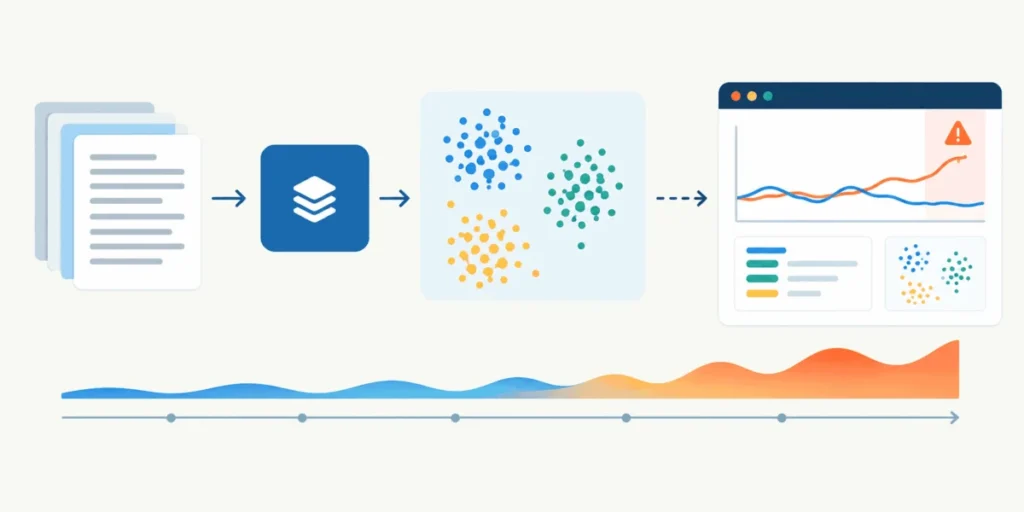
The deployment of a Large Language Model (LLM) into a production environment is rarely the finish line; rather, it is the beginning of a high-stakes lifecycle. As real-world user interactions unfold, the nature of incoming data inevitably shifts. Whether due to evolving cultural trends, seasonal changes in consumer intent, or the emergence of entirely new technical domains, the data a model processes today may look radically different from the data it was trained or fine-tuned on yesterday.

In the world of modern AI, this data is transformed into high-dimensional numerical vectors known as embeddings. When the statistical distribution of these embeddings deviates from the baseline established during development, we encounter "embedding drift." If left unmonitored, this drift can lead to degraded model performance, hallucinated responses, and a breakdown of user trust. This article explores the imperative of detecting embedding drift and provides a technical roadmap for implementing robust detection strategies.

The Core Challenge: Understanding Embedding Drift

At its heart, an LLM functions by mapping textual information into a dense vector space—a mathematical representation where similar concepts occupy neighboring regions. When a system is first deployed, engineers establish a "baseline" embedding distribution. This baseline represents the "known world" of the model’s expected inputs.

Embedding drift occurs when the incoming stream of user data forces the model to generate embeddings that occupy new, unchartered territories in that vector space. Unlike traditional tabular data monitoring, where a shift in a single column (like a change in median age or income) is easily observable, embeddings are opaque. They are high-dimensional arrays, often containing 384, 768, or even 1,536 dimensions. Traditional statistical tests, such as the Kolmogorov-Smirnov test, are often ineffective or computationally prohibitive when applied to such high-dimensional structures. Consequently, organizations must adopt specialized, machine-learning-centric approaches to detect when a model has lost its "alignment" with its intended use case.

Chronology of an LLM Failure: From Drift to Degradation

To understand the urgency of drift detection, one must visualize the typical degradation cycle of a production LLM:

1. Deployment (The "Honeymoon" Phase): The model is optimized for a specific domain, such as customer support for a SaaS platform. Accuracy is high, and latency is within acceptable bounds.
2. Gradual Shift: User queries begin to include new terminology. Perhaps a new product feature is launched, or a macro-economic event changes the nature of user complaints. The model still functions, but its internal embedding representations begin to "migrate."
3. The "Blind Spot": The model, trained on legacy data, fails to map these new, drifting embeddings to the correct intent, leading to decreased precision in retrieval-augmented generation (RAG) systems.
4. Performance Collapse: The model begins to output irrelevant or "hallucinated" answers. Users stop relying on the system, and the business value of the deployment erodes.

By implementing proactive drift detection, developers can intervene at the "Gradual Shift" stage, triggering retraining pipelines or fine-tuning sessions before the "Performance Collapse" occurs.

Proven Techniques for Detecting Embedding Drift

Effective monitoring requires a multi-layered approach. The industry has converged on several highly effective techniques:

1. The Domain Classifier Approach

This is arguably the most robust method for high-dimensional data. By training a secondary, lightweight "domain classifier"—often a Random Forest or a simple neural network—one can attempt to distinguish between "baseline" data and "production" data.

• The Logic: If the classifier can easily distinguish between the two sets (achieving a high ROC-AUC score), it implies that the datasets are fundamentally different.
• The Threshold: A score of 0.5 suggests the datasets are indistinguishable (no drift), while a score approaching 1.0 indicates a significant, measurable drift that necessitates intervention.

2. Centroid Distance (The "Center of Mass" Method)

This approach measures the distance between the mean vector (the centroid) of the reference data and the mean vector of the production data.

• The Logic: If the "average" position of incoming data has moved significantly away from the original center of mass, the model is likely processing a different distribution of concepts.
• The Limitation: While computationally efficient, this method sacrifices nuance. It can mask multi-modal shifts where data is moving in two different directions that happen to cancel each other out in the mean calculation.

Technical Implementation: A Practical Guide

To demonstrate these concepts, we utilize scikit-learn alongside scikit-llm and sentence-transformers.

Simulating Drift

First, we establish our baseline using numpy to generate a 384-dimensional space, mimicking the output of popular models like all-MiniLM-L6-v2.

import numpy as np
from sklearn.ensemble import RandomForestClassifier
from sklearn.model_selection import train_test_split
from sklearn.metrics import roc_auc_score

# Generate baseline data
n_samples = 500
n_features = 384
np.random.seed(42)
X_reference = np.random.normal(loc=0.0, scale=1.0, size=(n_samples, n_features))

# Simulate production drift by shifting the mean
X_production = np.random.normal(loc=0.3, scale=1.0, size=(n_samples, n_features))

Building the Domain Classifier

By combining these datasets and training a classifier, we can quantify the drift.

y_reference = np.zeros(n_samples)
y_production = np.ones(n_samples)
X_combined = np.vstack((X_reference, X_production))
y_combined = np.hstack((y_reference, y_production))

X_train, X_test, y_train, y_test = train_test_split(X_combined, y_combined, test_size=0.3)

drift_classifier = RandomForestClassifier(n_estimators=50, max_depth=5).fit(X_train, y_train)
roc_auc = roc_auc_score(y_test, drift_classifier.predict_proba(X_test)[:, 1])

if roc_auc > 0.65:
    print(f"ALERT: Significant drift detected (ROC-AUC: roc_auc:.3f)")

This classifier provides a clear signal, effectively acting as an "early warning system" for your production pipeline.

Implications for Modern Enterprises

The implications of ignoring embedding drift are not merely technical; they are financial and operational. For companies relying on LLMs for customer-facing applications, an unmonitored drift can result in:

• Increased Support Costs: As the model fails to provide correct answers, users escalate issues to human support agents.
• Compliance Risks: If a model drifts into discussing topics outside of its approved guardrails, companies may face regulatory scrutiny.
• Wasted Compute: Continuing to serve a model that is no longer performing accurately is a misuse of expensive GPU resources.

Official Perspectives and Best Practices

Leading AI safety researchers emphasize that monitoring is not a one-time setup but an ongoing requirement. "Drift detection is the observability layer of the AI era," says Dr. Elena Rossi, an AI infrastructure consultant. "Organizations must treat their embedding logs with the same rigor they apply to their database transaction logs. If you cannot measure the semantic drift, you cannot manage the model’s reliability."

Real-World Application: Using Scikit-LLM

When moving from simulation to real-world text, the implementation changes slightly. We must use a vectorizer to transform raw queries into embeddings. In this example, we use the SentenceTransformer library to bridge the gap between human language and machine-readable vectors.

from sentence_transformers import SentenceTransformer

# Load a local, lightweight vectorizer
vectorizer = SentenceTransformer('all-MiniLM-L6-v2')

# Define datasets representing a clear topic shift
texts_reference = ["How do I reset my password?", "Where is the billing menu?"] * 100
texts_production = ["The new crypto system is failing", "How to mint an NFT?"] * 100

# Convert to embeddings
X_reference = vectorizer.encode(texts_reference)
X_production = vectorizer.encode(texts_production)

# Proceed with domain classification as shown in the previous section

The result of this process is an ROC-AUC score of 1.000, confirming that the model has successfully identified that the incoming queries are fundamentally different from the training data. The centroid distance method, while simpler, will also confirm this shift, albeit with a different mathematical sensitivity.

Conclusion: Building a Resilient AI Future

Monitoring embedding drift is a foundational requirement for any organization seeking to derive long-term value from Large Language Models. By implementing domain classifiers and centroid monitoring, engineering teams can transition from reactive troubleshooting to proactive management.

As the AI landscape continues to accelerate, the ability to observe and interpret the shifting semantic landscape of your production data will define the leaders from the laggards. It is not enough to simply launch a model; one must ensure that the model remains a relevant, accurate, and stable asset throughout its entire operational life. By integrating the techniques outlined here, you can build an infrastructure that is as dynamic and adaptable as the user base it serves.