Demystifying the Vector Database: A Ten-Step Journey from Theory to Implementation
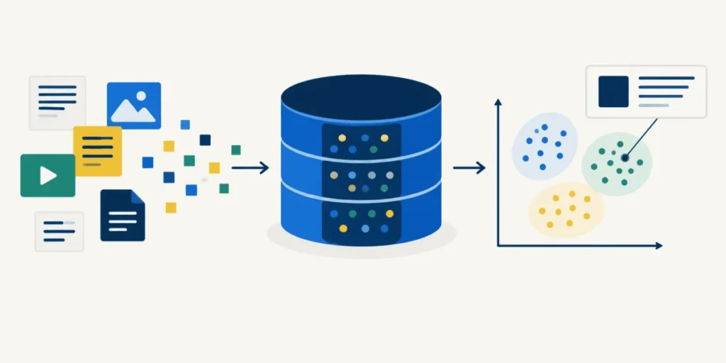
In the rapidly evolving landscape of artificial intelligence, vector databases have emerged as the "long-term memory" for Large Language Models (LLMs). While enterprise-grade solutions like Pinecone, Milvus, and Weaviate dominate the market, the underlying mechanics of how these systems function are often shrouded in complexity. To truly understand the engine driving modern semantic search, one must look past the APIs and into the core mathematical operations.
By utilizing Python and the powerhouse library NumPy, developers can strip away the abstraction layers to reveal the elegant, surprisingly simple architecture that allows machines to "understand" context rather than merely matching keywords. This article breaks down the construction of a functional vector database into ten incremental steps, demonstrating that the leap from a basic script to a scalable search engine is far smaller than commonly perceived.
The Paradigm Shift: Beyond Keywords
Traditional databases rely on keyword matching—a brittle approach that fails the moment a user employs a synonym or a slightly different phrasing. Vector databases operate on a different philosophy: semantic proximity. By converting text into high-dimensional vectors—arrays of numbers that represent the underlying "meaning" of the content—we can perform geometric calculations to determine how closely related two pieces of information are.
When a query is submitted, it is also converted into a vector. The database then calculates the "distance" between the query vector and the document vectors in the index. The closer the vectors point in space, the more relevant the result. This tutorial requires no GPU and no expensive API keys; instead, it relies on local embedding models and the raw, efficient computational power of NumPy.
Chronology: The Ten-Step Construction
To follow this architectural journey, you should set up a workspace with three primary files: vector_db.py (the engine), corpus.py (the data source), and test.py (the verification suite).
1. The Foundation and Setup
The process begins with installing numpy and sentence-transformers. By initializing a script, we define two critical helper functions: header() for formatting and show() for rendering results. At this stage, the database is an empty shell; we are establishing the interface through which we will interact with our data, ensuring that search results include the similarity score, topic metadata, and the document snippet itself.
2. Indexing the Corpus
When we initialize our VectorDB class, we load an embedding model. The add() method is where the heavy lifting happens: it transforms each text document into a fixed-length vector of 384 dimensions. This is a crucial design choice. Regardless of whether a document is a single sentence or a multi-page essay, the resulting vector remains a flat, 384-element array. This predictability is what makes vector indexing computationally efficient and memory-stable.
3. The First Semantic Query
We start by asking: "What keeps a cell supplied with energy?" A standard keyword-based search might struggle with this, but our vector database identifies "mitochondria" as the powerhouse of the cell, even though the query didn’t explicitly use that word. The search is driven by the latent semantic relationship encoded during the embedding process.
4. Navigating Concepts Without Keyword Overlap
The true power of vector search is demonstrated when a query shares no words with the target document. For instance, querying "why does my loaf taste sour" retrieves documents about sourdough fermentation and lactic acid bacteria. There is zero lexical overlap, yet the system identifies the intent perfectly. This is the hallmark of modern semantic retrieval.
5. Interpreting Similarity Scores
Not all results are equal. A vector database returns a list of results ranked by a similarity score. By comparing the high scores of relevant matches to the lower, less relevant scores of unrelated content, we learn the importance of setting a "threshold" in production environments to filter out noise.
6. Metadata Filtering: Adding Constraints
Similarity is not always enough. Sometimes, a document is semantically relevant but contextually wrong—like a comic book character’s "mitochondria-rich muscle fibers" appearing in a biology search. By using metadata tags (e.g., "topic": "bio"), we can constrain the search space, ensuring that the engine only ranks documents within the desired domain.
7. Refining the Filter Logic
Step seven illustrates that metadata filtering acts as a pre-processing gate. If a user asks for five results within the "music" category, and only one exists, the system correctly returns only that one. This prevents the "padding" of results with irrelevant content, maintaining high precision.
8. Implementing Guard Rails
Building a robust system requires handling user error. By adding checks to ensure that input types are correct and that metadata entries align one-to-one with documents, we prevent silent data corruption. These guard rails are essential for maintaining the integrity of the index.
9. Persistence: Saving and Loading
An index is only useful if it can be saved. We store our vectors in a .npy file for compact, high-speed binary storage and our metadata in a .json file for readability. Crucially, the system includes a safety check: you cannot load an index created with a different embedding model, as the underlying numerical "language" would be incompatible.
10. Measuring Scalability
Finally, we test the performance using a synthetic corpus of 100,000 vectors. We find that the scan time remains remarkably low, proving that the architecture is not just a toy project, but a robust framework that can scale significantly before requiring advanced optimizations like approximate nearest neighbor (ANN) indexing.
Supporting Data and Technical Analysis
The efficiency of this system is derived from the "cosine similarity" calculation. By normalizing our vectors to a length of 1, the similarity calculation simplifies to a basic matrix multiplication (rows @ query_vector). This allows us to process thousands of comparisons in milliseconds.
The following table summarizes the performance benchmarks observed during the scaling test:
| Documents | Memory Usage | Scan Time (ms) | Rank Time (ms) |
|---|---|---|---|
| 1,000 | 1.5 MB | 0.01 | 0.04 |
| 10,000 | 14.6 MB | 0.36 | 0.55 |
| 100,000 | 146.5 MB | 3.73 | 8.90 |
These results demonstrate that as the dataset grows, the time taken to perform a search increases linearly. While this is acceptable for tens of thousands of records, it highlights why specialized enterprise databases eventually move toward tree-based or graph-based indexing to keep search times constant even as they scale to millions of records.
Implications for Future Development
The construction of this database provides three major takeaways for developers:
- Simplicity is Scalable: The core logic of a vector database—matrix multiplication—does not change whether you have 25 or 25 million documents. The complexity lies in the management and indexing strategies surrounding that core.
- Model Sensitivity: The index is inextricably tied to the model that created it. This underscores the necessity of robust version control for embedding models; changing the model invalidates the entire database.
- Semantic Reliability: By moving away from keyword matching, we enable systems to handle natural language queries with a level of nuance that was impossible a decade ago. This shift is the bedrock upon which current RAG (Retrieval-Augmented Generation) architectures are built.
Conclusion
Building a vector database from scratch is an exercise in demystification. It proves that the "magic" of AI-driven search is firmly rooted in linear algebra. By mastering the fundamental steps—embedding, indexing, filtering, and persisting—developers gain the ability to build sophisticated, context-aware applications without necessarily relying on black-box proprietary services. As the ecosystem continues to mature, understanding these foundational mechanics will remain a vital skill for any engineer looking to harness the true potential of machine learning.